Mathematically, given a probability space \( (\Omega, \mathcal{F}, \mathcal{P}) \), a real-valued stochastic process \( \{W_t : t \geq 0\}\) is a standard Wiener process if it is characterised by the following properties:
Therefore, by definition, the Wiener process has stationary and independent increments. The latters are normal random variables, which means that they can have both positive and negative real values. The previous two properties are called distributional properties. Another property is the closure properties, meaning that if you apply some operations to it, you obtain another Wiener process. For example, suppose you have the Wiener process \( W = \{W_t : t \geq 0\}\), and you scale it for a certain costant \(c \gt 0\), then \( \{W_{ct}/\sqrt{c} : t \geq 0\} \) is still a Wiener process. Regardin the sample pahts of this stochastic process, they are continous almost everywhere (almost everywhere := the only region where the property does not hold is mathematically negligible).
An important derivation of the Wiener process is the geometric Brownian motion (GMB), a continous-time stochastic process, where the logarithm of the variable subject to random fluctuations follows a Brownian motion with drift. More precisely, a stochastic process \(S_t\) follow a GMB if it satisfies the following SDE: \[dS_t = \mu S_t dt + \sigma S_t dW_t\] where \(W_t\) represent the Wiener process while \(\mu\) and \(\sigma\) denote the drift and volatility, respectively.
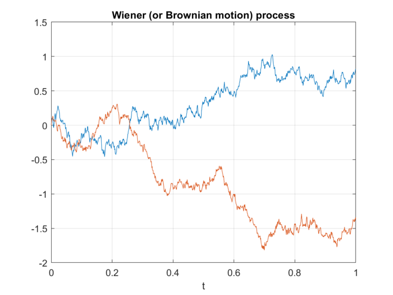
In the following graph a simple random walk simulate the Brownian motion, a mathematical model for random movements observed in various natural phenomena. A particle starts at the center and takes random steps inboth horizontal and vertical directions.